1 Introduction

Since the sixties it has been suggested that the analysis of volcano repose intervals (or inter-event times, IETs) can be used to forecast eruptions (e.g., Wickman, 1966; Klein, 1982; Mulargia et al., 1985). Since then, several studies have followed this approach, and have proposed different probability distributions to model repose intervals, starting from the simple exponential model for Poisson processes (e.g., De la Cruz-Reyna, 1991; Marzocchi and Zaccarelli, 2006), to other models characterized by more parameters, such as:

• Failure models based on the Weibull distribution (e.g., Voight, 1989; Bebbington and Lai, 1996), which assumes the probability of event occurrence varying since the time of the last event, and in particular it may increase/decrease based on the value of the shape parameter.

• LogLogistic models (Connor et al., 2003), which describe the influence of two competing processes, one increasing and one decreasing the probability of an event with time from last event.

• Power-law models, characterized by possible infinite variance and mean (Pyle, 1998).

• Self-exciting models for the event rate (also called intensity in literature), in which every event increases the likelihood of a subsequent event, but this influence decreases with time (Bebbington and Cronin, 2011; Bevilacqua et al., 2016).

• Brownian Passage Time (BPT) model, characterized by a parameter indicating the mean repose time and an “aperiodicity” parameter, measuring the aperiodicity of the mean response of the system (Garcia-Aristizabal et al., 2012; Garcia-Aristizabal et al., 2013); this model has proved useful to compare different systems spanning from periodic-like to Poisson-like (aperiodic) systems, and has an asymptotic (long-term) finite and constant hazard function toward infinite times;

• Lognormal models, usually describing a quasi-periodic behavior (Bebbington and Lai, 1996).

• Mixtures of some of the above distributions, as e.g., mixture of exponentials (Mendoza-Rosas and la Cruz-Reyna, 2008) or mixture of Weibulls (Turner et al., 2008), to describe multi-modal processes.

All these models assume that the repose intervals in a given catalog are a sample from a common parent distribution that governs a stationary (that is, the parameters of the parent distribution do not change over time) process generating the data.

However, a frequent characteristic of volcanic activity is its tendency to concentrate during temporal frames, that is, to occur in temporal clusters. This has been studied in several papers (e.g., Conway et al., 1998; Cronin et al., 2001; Bebbington, 2010; Bevilacqua et al., 2016) in different volcanic settings. In these models there is no specific objective identification of possible groups of events (or clusters) that are sometimes observed in the real datasets. In other words, clustering in these models may appear as a consequence of the nature of the parent distribution; for example, a process described by a Weibull distribution may exhibit a degree of clustering (in case the shape parameters is smaller than 1), as well as self-exciting models.

Another development in the modeling of repose time intervals is to include also the size of eruptions, parameterized by the erupted mass, erupted volume, or the eruption magnitude (Pyle, 2000) or by the VEI (Newhall and Self, 1982). For example, several studies have searched for a significant link between sizes of eruptions and their subsequent repose times, that is known as Time-Predictable Model (TPM), or between repose times and the sizes of their subsequent eruptions, that is known as Size-Predictable Model (SPM), both in the classical (De la Cruz-Reyna, 1991; Burt et al., 1994) or in a generalized form (e.g., Sandri et al., 2005; Marzocchi and Zaccarelli, 2006; Bebbington, 2008; Passarelli et al., 2010; Garcia-Aristizabal et al., 2012; Sandri et al., 2017). These models have the advantage of providing a simple conceptual model linking the repose time intervals to the process of loading and discharging of the magma storage system.

Finally, in analogy with the famous Gutenberg-Richter law in seismology (Gutenberg and Richter, 1944), when a catalog of eruptions from a volcano is available, one may also wonder how to model the distribution of eruption magnitude occurrences, in a so called frequency-size law.

A new up-to-date catalog for Galeras volcano has been recently collated by integrating official catalogs from the Colombian Geological Survey and data from the Smithsonian Institution. The main goal of this paper is to provide a statistical description of the main features of the eruptive activity at Galeras volcano (Colombia), and to better understand the processes generating the observed data. This goal is achieved by applying the methodologies described above.

We analyze the Galeras' new catalog in different perspectives: the temporal domain, the magnitude domain, and the time-magnitude domain. In general, we mostly use standard statistical analyses to describe the volcano's eruptive behavior; moreover, we adapt these analyses in order to obtain clues about eruption recurrence considering clustered processes.

The paper is organized as follows: first, we give a brief introduction about the volcanic setting of Galeras (Section 2), and about the new eruption catalog, with the preliminary study to find adequate thresholds in time and magnitude to consider the catalog as complete (Section 3). Then, in Section 4 we describe the methods we use to analyze the catalog in the three perspectives; in particular:

• In Section 4.1 we search for the best recurrence model describing the IETs distribution, both by taking all the eruptions as single events and by means of cluster analysis to objectively identify and analyze clusters of eruptions. With these models, we aim at describing the main features of Galeras' catalog. In particular, with the cluster analysis, we would like to assess how likely it is that a future eruption belongs to an already-ongoing cluster, or marks the start of a new one;

• In Section 4.2 we model the frequency-size relationship;

• In Section 4.3 we search for significant links between the repose times and the magnitudes of eruptions in the Galeras catalog, in order to reject or not the hypothesis of a significant time- or size-predictability in the data.

We present the results of our analyses in Section 5, following the same logical order as in Section 4. Finally, in Section 6 we discuss and compare the results obtained in the three perspectives with the aim of trying to understand better the magma feeding system of Galeras volcano.

2 Galeras Volcano

Galeras volcano is an andesitic stratovolcano 4200 m high, located at 1.221^°N and 77.359^°W in southern Colombia, close to the Colombia-Ecuador border (Calvache, 1990; Hurtado Artunduaga and Cortés Jiménez, 1997; Cepeda, 2020). According to Calvache et al. (1997) Galeras volcano is located in the scar left of the former Urcunina stage collapse, which left an amphitheater that opens toward the west, the active cone being the current Galeras volcano stage. The eruptive activity at Galeras volcano, which began about 5.000 years ago (Calvache, 1990; SGC, 2015), is mainly characterized by relatively small-volume, vulcanian eruptions (Hurtado Artunduaga and Cortés Jiménez, 1997).

Historical records of Galeras volcano activity only began after the Spanish colonization. Stories of the chroniclers resulted in an almost complete record of historical eruptions (Calvache, 1990) since the 16th century. Most of the eruptions occurred in the$\sim$500 years of historical record can be considered to be explosive of small to moderate in size (Bonadonna and Costa, 2013), with some of them accompanied by small pyroclastic flows (Espinoza, 1988; Hurtado Artunduaga and Cortés Jiménez, 1997). However, the risk for the population can be high, as almost 500,000 people inhabits in the proximity of the active crater (DANE, 2011) and more than 5,000 people live within the high hazard zone (UNGRD, 2019).

3 Data and Definition of a Complete Data Set

3.1 Collation of the Explosive Eruptive Events Database

Galeras is one of the most active volcanoes in Colombia (Calvache, 1990). A considerable number of eruptions at Galeras has been recorded and identified in the last 5,000 years. Although, as mentioned above, the majority of these events has been generally characterized by vulcanian activity, at least six major events have been recognized and analyzed (Calvache et al., 1997). The third version of hazard map of Galeras volcano considers a total of 45 events found in stratigraphic records (Hurtado Artunduaga and Cortés Jiménez, 1997). An additional catalog of historical records of the last 500 years registered by numerous authors (Calvache, 1990) was compiled and documented by Espinoza (1988).

The catalog of Explosive Eruptive Events (EEE) used in this work was produced integrating geological and historical information obtained from different sources (Calvache, 1990; Hurtado Artunduaga and Cortés Jiménez, 1997; Stix et al., 1997), including the Smithsonian Institution catalog (Global Volcanism Program, 2013) and data from the Colombian Geological Survey (formerly INGEOMINAS), who provide detailed reports of the last periods of activity (INGEOMINAS, 2005; INGEOMINAS, 2010). A total of at least 78 eruptive events were registered between 3120 BCE and 2010 CE. Furthermore, the catalog includes calculated data as eruption date, VEI, magnitude, and, for recent eruptions, the volume and column height.

Smithsonian Institution and Colombian Geological Survey were the primary sources of the data. Both offer a catalog of the events and provide mainly information about the eruption date and the VEI value. Other characteristics as mass, volume, and column height were taken also from complementary sources (Calvache, 1990; Hurtado Artunduaga and Cortés Jiménez, 1997; Stix et al., 1997).

However, the information available for some eruptions (in general the older ones) is derived from historical descriptions that do not include technical details or the exact date; in these cases, where possible, the missing information was inferred using relationships among parameters available in the literature (i.e., Newhall and Self, 1982). The final EEE catalog produced in this work is provided in the Supplementary Material (Section Supplementary Material).

In order to proceed with catalog analysis, we fill in the missing months and/or days with random dates, without altering the recorded succession of events. If only the day is missing, we pick a random day in that month; if also the month is missing, we pick a random day in the year. To check the influence of this choice, we also filled in the missing dates by using the mid point of the missing period with no difference in the obtained results.

3.2 Defining a Complete Dataset in Time and Size

To study the temporal pattern of EEEs occurrence it is necessary that the input catalog represents a complete record of events above a given size, avoiding bias in the analysis by possible under-reporting of events. Therefore, we first analyze the completeness of our dataset by looking for significant changes in the rate of events in time.

By considering both the whole data (Figure 1) and the subset of events with magnitude M $\ge$ 2.6 since 1820 (Figure 2), we notice that the increase in event rate since the 1820s may indicate a bias due to the under-recording of small magnitude events before then. For this reason, we consider as complete the catalog since 1820s only for events above or equal to magnitude 2.6, and these time and size constraints are used to set the dataset to be analyzed in this paper. In doing so, we realize we are discarding the largest portion of the most recent recorded events (approximately since 1990), which probably represents the most accurate record of what has happened at Galeras, complete for much lower magnitude. However, on the one hand we cannot use only the latter 30-years data to infer the long-term behavior of the volcano, as we would end up with too few events to conduct a sound statistical analysis, representative for a short period of time; on the other hand, as reported in Section 4.2, we use this last 30-years portion of the catalog to build a frequency-size distribution that is then compared with the results obtained using the longer-term, complete catalog.

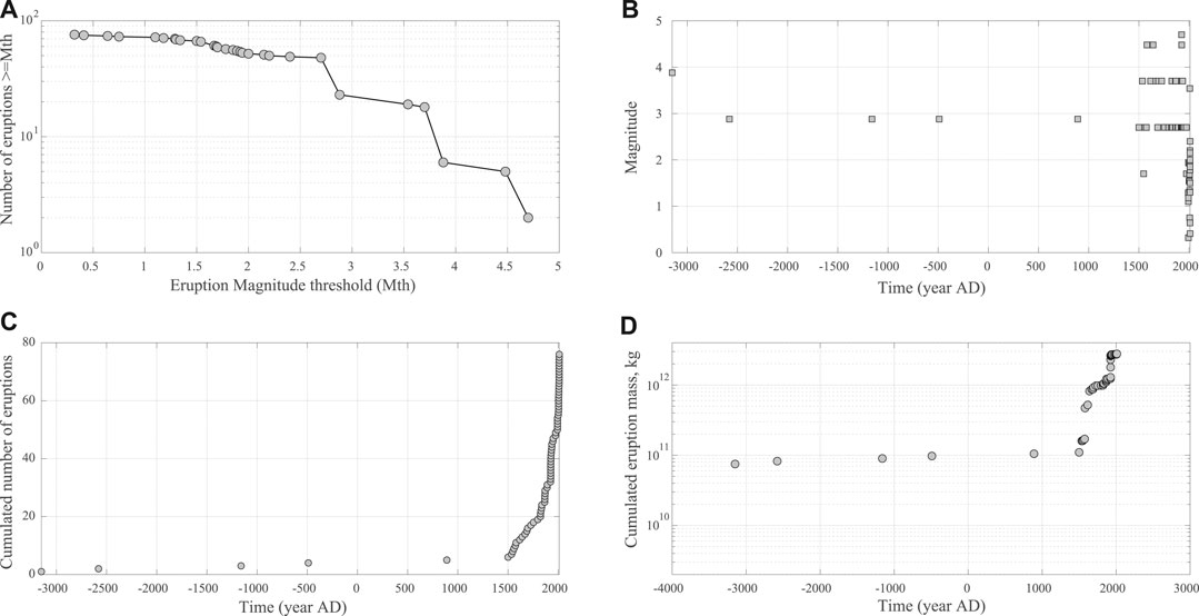
FIGURE 1. Galeras's new catalog collected, since 3000BP. (A): the frequency-size plot (B) time series of eruption occurrence and magnitude; (C) Cumulative Distribution Function of onset times of all events in catalog (D) Cumulative erupted mass in time.

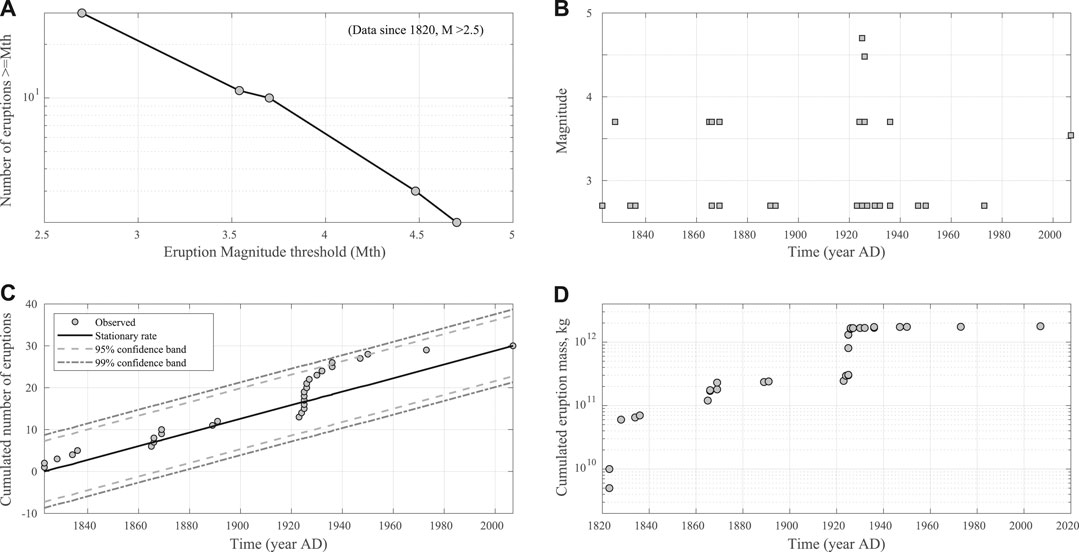
FIGURE 2. Same as Figure 1, for the complete part of the catalog only, i.e. only eruptions of M $\ge$ 2.6 since 1820AD. In panel C we also show the theoretical relationship (solid line) for a perfect stationary process, while the dashed/dashed-dotted lines show the $95/99\%$ confidence interval.

4 Modelling Approach

4.1 Temporal Analysis

One of the aims of this paper is to study the temporal distribution of EEEs at Galeras volcano. In Figure 2C we plot the cumulative number of EEEs at Galeras in time; a visual inspection of this plot may indicate their possible temporal clustering, in which explosions exhibit a tendency to form groups of events close in time. Figure 2D shows the cumulative erupted mass (in kg) as events occur in the complete part of the catalog. A visual inspection of this plot suggests also a possible relationships between the repose times between subsequent events and the erupted mass in one of the two events.

Keeping in mind these observations, in this paper we analyze the catalog of eruptions of Galeras volcano from different perspectives; in practice, we perform a dual analysis by studying in parallel recurrence features of single EEEs (we informally call this analysis “all IETs together”), and groups of EEEs occurring close in time, that hereinafter we call clusters. Beyond a classical recurrence analysis of eruptions, we are interested in examining the behavior of the clusters.

4.1.1 Recurrence Analysis of Single EEEs (“all IETs Together”)

As a first step we perform a classical recurrence analysis considering the complete part of the catalog. With this aim, EEEs are treated as a stochastic point process in which individual occurrences are assumed to be independent random events in time, at times $t_1<t_2<\dots <t_i\dots$. We define IETs, the time passed between two consecutive EEEs, as ${\tau }_i=t_{i+1}-t_i$, $\left(i=\mathrm{1,2},\dots \right)$. Adopting this approach, and ignoring the event duration, implies assuming that the EEE onset time is the most physically meaningful information (Garcia-Aristizabal et al., 2012); therefore, our modeling aims to describe the waiting times of the physical processes governing renewed volcanic activity.

In order to fit our complete dataset with renewal models, the data need to be first checked for stationarity (i.e., generated by a stationary process) and independence (i.e., successive IETs must be independent). Thus, we check independence between successive IETs of events in the complete part of the catalog by rejecting a correlation between the duration of successive IETs as in Bebbington (2012). Further, we check stationarity in the IET-generating process (in the complete part of the catalog) by running the Kolmogorov-Smirnoff test to reject significant deviations from a uniform distribution of the onset times of events.

In the light of these tests, the complete part of the catalog, consisting of independent IETs generated by a stationary process, is described by considering alternative renewal models. The performance of the different statistical models is evaluated through the Akaike Information Criteria (AIC), trying to find a good balance between goodness-of-fit to the data and model simplicity (expressed by the number of free parameters). In particular, if our IETs can be taken as a sequence of random variables $\left\{\tau \right\}$ independent and distributed according to a function $F\left(\tau \right)$, then the original series of events $\left\{t_i\right\}$ is called a renewal process. To better understand the nature of these competing models (and in particular the preferred one based on the AIC), we calculate and plot the hazard rate, which for a history-dependent point process is the ratio of the probability density function $f\left(x\right)$ to the survival function S(x):

$H\left(x\right)$ is the instantaneous event rate at time t conditional on survival until the time t, with $x=\left(t-t_L\right)$, being $t_L$ the occurrence time of the last event before t (e.g., Bain, 1978).

The renewal models that we test are the Exponential, the Weibull, the LogLogistic, the Lognormal, the Gamma and the Brownian Passage Time (BPT). Except the Exponential distribution, characterized by one parameter, these statistical models are described by two parameters (see Table 1). Further, we also test a mixture of Exponentials (3 parameters) and a mixture of Weibulls (5 parameters), in analogy with previous works (e.g., Turner et al., 2008), trying to explain a possible bimodality in the set of the IET taken all together. In order to fit the two latter models, we implemented a Markov chain Monte Carlo (MCMC) approach; however, we check the consistency of the results using also the algorithms provided by Bebbington (2012). In fitting these models vs. the cataloged data, we also use the censoring information, i.e., no $M\ge 2.6$ event has occurred since October 4, 2007, up to the end of 2019.

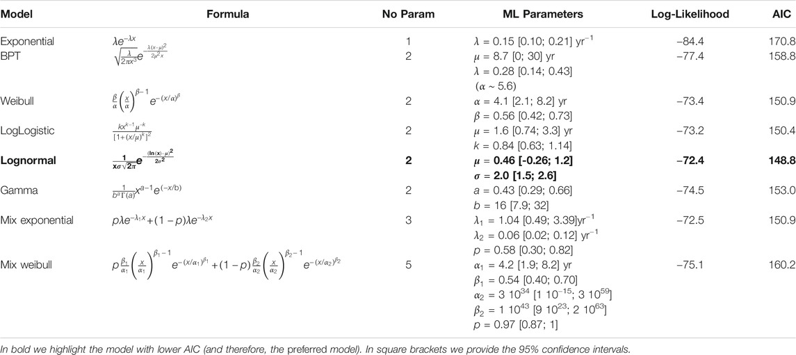
TABLE 1. Renewal models fit to the IETs data (x in years), considering the censoring information of no failure at the date of December 31, 2019.

4.1.2 Recurrence Analysis Assuming Clustered Eruptions

Observing the Galeras data set and the value of the Coefficient of Variation of the IETs, equal to 1.65 (e.g., Marzocchi and Zaccarelli, 2006), it seems plausible that EEEs exhibit some degree of clustering in the time domain. For this reason, we hypothesize the possibility that, once a new event or a new eruptive cycle starts, the short-term behavior of the eruptive activity may follow different patterns during the evolution of the activity.

Therefore, in alternative to the data analysis proposed in the previous paragraph, we may hypothesize the possibility of two different processes governing the behavior of eruptive activity in the time domain: a) a long-term process that determines the recurrence of eruptive cycles (or eruption clusters), and b) a short-term process that determines the recurrence of eruptive activity within each eruptive cycle (once it has started). From a stochastic point of view, we analyze this problem by considering these two processes as follows: in the long-term, eruptive activity can be described by the onset of eruptive cycles (i.e., clusters), and the stochastic characterization of such processes can be described by analyzing the rate at which these eruptive cycles take place. In the intra-cycle time scale, once an eruptive cycle has started, the eruptive activity can be described by analyzing the occurrence of events within the eruptive cycle. For this analysis, we select the complete part of the eruptive catalog identified by the methods described in the previous section. Then:

• First, we identify plausible data set partitions to form event clusters. This analysis can be performed by hand processing (e.g., if the data clearly shows these partitions), or adopting a more quantitative approach based on any cluster analysis technique. Although the Galeras eruptions somehow exhibit clear groups of eruptions in the time domain that could be identified as clusters, we adopt a classical partitioning approach using the k-means method (MacQueen, 1967), which is described in the following paragraphs.

• Once the clusters are identified, we set the start time of each cluster by selecting the time of the first event within each cluster. Such cluster start times are used to compute the inter-cluster time intervals.

• The inter-cluster time intervals are analyzed by testing different renewal models (the same as above: Exponential, Weibull, LogLogistic, Lognormal, Gamma and BPT); the most adequate distribution is again selected by using the AIC.

• For the events within each cluster, we calculate the intra-cluster IETs, that are the time intervals between the events belonging to the same cluster. Again, such IETs are analyzed by testing different renewal models and the most adequate one is selected by using the AIC.

4.1.2.1 Cluster Analysis

The k-means algorithm used for cluster analysis (MacQueen, 1967) takes the input parameter (k), which represents the number of clusters, and partitions a set of n objects into k clusters so that the resulting intra-cluster similarity is high compared to the inter-cluster similarity.

Defining an adequate number of clusters k is a challenging issue (see e.g., Garcia-Aristizabal et al., 2017); in this work we use the popular Silhouette Method (Rousseeuw, 1987; Xu and Wunsch, 2005; Al- Zoub and al Rawi, 2008; Kaufman and Rousseeuw, 2008). Given a partition into k clusters, this method assigns a silhouette coefficient to every object in the dataset; this coefficient depends on i) the average distance between the object and the objects belonging to its cluster, and ii) the average distance between the object and the objects belonging to other clusters. For a satisfactory partitioning, the latter must be larger than the former, and in this case the coefficient takes positive values.

The unknown optimum k value is the one in which all the silhouette coefficients in each cluster:

• Are positive (otherwise it means either there is an “outlier” object in the cluster that is very far from its “companion” objects), and

• Are all comparable with the average silhouette value of all clusters (otherwise it means there is a cluster that is not clearly separated from another one).

The silhouette method offers the advantage that it only depends on the actual partition of the objects, and not on the clustering algorithm that was used to obtain it. Its usefulness in the interpretation and validation of cluster analysis results has been discussed in a number of applications (e.g., Rousseeuw, 1987; Chen et al., 2002; Bolshakova and Azuaje, 2003; Garcia-Aristizabal et al., 2017).

4.2 Frequency-Size Analysis

In the previous paragraphs we presented the methods for analyzing the distribution of Galeras eruptions in the time domain considering both single and clustered eruptions. However, determining a frequency-magnitude (F-M) relationship for natural phenomena is another key issue for hazard and risk assessments since it allows one to estimate the return period of damaging events. As for other natural hazards, the frequency of explosive eruptions decreases as their size or magnitude increase; while for some phenomena (as e.g., earthquakes, extreme meteorological events, or flooding) there exist event catalogs populated with enough data for quantitative analyses, the record of eruptions from a single volcano is usually composed by a few events for which it is often difficult to properly define a F-M model. For this reason, the most sound F-M models proposed to describe the distribution of eruption magnitudes rely on regional to global analyses in which large eruptions from different volcanoes are merged and generalized in a single model (e.g., Simkin and Siebert, 2002 onwards). However, it is worth to note that while such aggregations may show an identifiable F-M distribution, it is not implied that this relationship holds for any particular volcano.

In this context, different F-M models for describing volcanic explosions have been proposed in literature, which are based, for example, assuming a exponential magnitude distribution (similarly to the Gutenberg-Richter model in seismology, as e.g., De la Cruz-Reyna, 1991; Mendoza-Rosas and la Cruz-Reyna, 2008), which is equivalent to assuming a power law distribution of eruption volumes (e.g., Papale, 2018) or mass, and it implies a so-called scale invariance in the eruption magnitude. Others authors have used extreme value theory (e.g., Mason et al., 2004; Coles and Sparks, 2006; Mendoza-Rosas and la Cruz-Reyna, 2008; Deligne et al., 2010; Furlan, 2010; Sobradelo et al., 2011).

In this study we try to fit our data with a power law describing the erupted mass $m_e$ in single events:

where $N\left(m\right)$ is the number of eruptions with erupted mass equal to m, and k and b are parameters of the law. By taking the logarithm of this equation, we get to the formulation that is similar to the Gutenberg-Richter law for earthquakes, i.e.:

where M is the magnitude of an eruption, which is a linear function of $Log\left(m\right)$ (Pyle, 2000). If this holds, magnitudes obey to an exponential distribution (Aki, 1965; Marzocchi and Sandri, 2003):

where $x=M-\left(M_c-\text{Δ}M/2\right)+\text{ε}$, being $M_c$ the completeness magnitude in the catalog, $\text{Δ}M$ is the magnitude bin (in our case 0.1 to 1), and ε is uniform random noise over $\left[-\text{Δ}M/2,\text{Δ}M/2\right]$ mimicking the magnitude uncertainty.

In this study, we follow the approach of Marzocchi et al. (2016), that basically consists of:

• Selecting a completeness magnitude $M_c$

• Testing (by a Lilliefors test, Lilliefors, 1969) the null hypothesis that eruption magnitudes are consistent with an exponential distribution; we need to apply a random noise ε to magnitude values, since they are binned to first decimal, thus introducing “fake” ties in the dataset, that alter the Lilliefors-test results

• if the null hypothesis is not rejected at 5% significant level, we fit the magnitude data with the maximum likelihood method (Marzocchi and Sandri, 2003) to estimate the b-value

Since we have already estimated the completeness magnitude in Section 2, we apply the scheme above for the data from 1820 and $M\ge 2.6$. However, since we also recognize a lower completeness magnitude if we reduce the catalog to the last 30 years (in particular, from 1990 with $M\ge 1.5$, see bottom panel in Figure 3) we repeat the above analysis also for this different dataset, which shares only one eruption (October 4, 2007) with the one from 1820 and $M\ge 2.6$. If we cannot reject the hypothesis of magnitudes following an exponential distribution for both datasets, we may compare the two b-values obtained and see whether they are consistent: in a scale-invariant process, they should have a unique value.

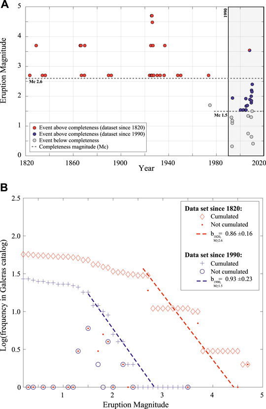
FIGURE 3. Frequency-size analysis: in red the S1 data (see text), i.e., from 1820, $M\ge 2.6$; in blue S2, i.e., from 1990, $M\ge 1.5$. In panel A we show the two datasets used (gray points are not used as they are below the completeness threshold); in panel B red dots and diamonds show respectively the not-cumulative and cumulative occurrences for S1 data, while blue circles and plus signs respectively show not-cumulative and cumulative occurrences for S2 data. The best fitting b-value lines are superimposed to the cumulative data, although they have been computed on the not-cumulative ones for an unbiased estimate.

4.3 Time-Predictable and Size-Predictable Models

The recurrence analyses presented so far provide important clues regarding the stochastic behavior in time of eruption events above the minimum completeness magnitude of eruptions. Complementary to such analyses, it is possible to explore the predictive value of other data in the catalog, in particular the possible relationships between the size and the time interval between eruptive activity. Such kind of models are generally referred to as time-predictable and size-predictable (e.g., De la Cruz-Reyna, 1991; Burt et al., 1994; Passarelli et al., 2010; Sandri et al., 2017).

We test such models for both the individual eruptions and the clustered eruptions. Regarding in particular the clustered data, on the complete part of the catalog partitioned in clusters, we calculate the total erupted mass within each cluster (taken as an eruptive cycle); afterward, we analyze this information considering the time preceding or the time following the respective eruptive cycle (taken as the time between the end of a cluster and the onset of the following one), searching possible significant relationships typical of time- or size-predictable systems.

Here, we generalize the classical conceptual models at the basis of time- or size-predictable systems as in Passarelli et al. (2010), by treating clusters as eruptive cycles, and searching for relationships between the “size” of a magmatic cycle (parameterized by the total erupted mass in the cycle) and the time elapsed from/to the previous/following cycle. We explore both classical linear relationships (as in De la Cruz-Reyna, 1991; Burt et al., 1994), as well as more general ones, such as a power law (as in Passarelli et al., 2010). In this view, any significant relationship between the total mass erupted in the preceding cycle and the time to subsequent eruptive cycle can be taken as a generalization of time-predictability. Conversely, any significant relationship between the time from the preceding eruptive cycle and the total mass erupted in the subsequent cycle can be taken as a generalization of size-predictability.

5 Results

5.1 Temporal Analysis

5.11 Recurrence of Single Eruptive Events

We analyze the time series of the IETs from 1820s above magnitude 2.6, to exclude any significant dependency between successive IETs of events with M ≥ 2.6 (Figure 4). We reject any significant correlation between the duration of successive IETs, both in terms of linear correlation (Pearson coefficient $r^2$ = 0.08, p-value $\gg 5\text{\%}$) and rank correlation (Spearman coefficient ρ = 0.34, p-value $>5\text{\%}$).

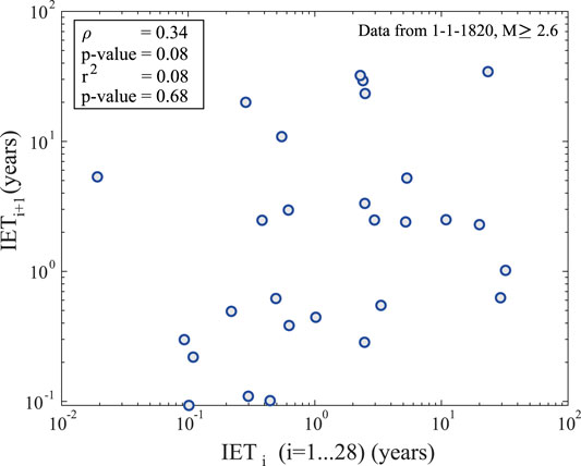
FIGURE 4. Independence of pairs of successive IETs.

The stationarity Kolmogorov-Smirnoff test on events with M ≥ 2.6 since 1820 (Figure 2C) is not rejected at 1% significance level (value of test statistics is 0.25), and we see that our data are well within the 99% confidence level. Thus, we do not reject the hypothesis that our data represent a stationary time series.

In the light of these tests, we take the list of events with M ≥ 2.6 since 1820 as a complete dataset, composed by independent IETs generated by a stationary process, and we fit it with the most common and simple renewal models (Figure 5), listed in Table 1 (where we show the models tested, their maximum likelihood parameters, and their AIC value). According to the AIC, the best model that describes the IETs of all the eruptions in the complete catalog is the Lognormal distribution (in bold in Table 1).

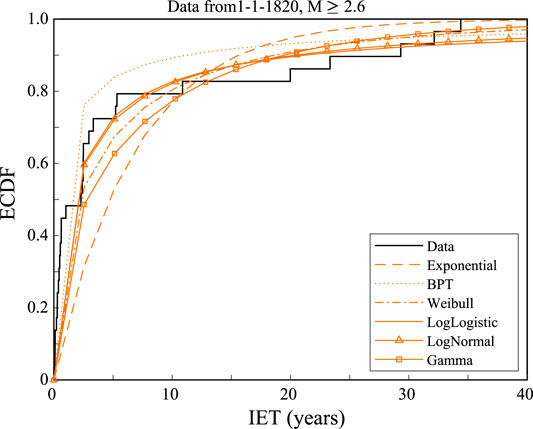
FIGURE 5. Model fit to the ECDF of IETs from events with M $\ge$ 2.6 since 1820s.

The mixture of exponentials with the best AIC shows an intermediate degree of mixing $\left(p=0.6\right)$ between two different exponentials, and explains the data certainly better than the single exponential (see Table 1); however, its AIC is not better than the one achieved by the Lognormal distribution.

The mixture of Weibulls fit by our MCMC algorithm systematically points toward solutions with the p parameter close to one; such solutions imply the prevalence of one of the Weibull components, which is characterized by the same parameter values of the single Weibull reported in Table 1. On the other hand, the fitting procedure by Bebbington (2012) points to an alternative solution with a good AIC but characterized by one of the two Weibull distributions being close to a Dirac delta, i.e., very peaked and not useful to understand any process generating these data. The difficulty to fit this model probably arises because of a complex likelihood surface (characterized by 5 parameters) to be maximized, making it hard to find a proper solution to the problem with the few tens of data available; ultimately, this may be related to a difficulty in discriminating between two processes hardly distinguishable with the data at hand. Thus we conclude that the mixture of Weibulls is not helpful in our case, and that our best model when considering all the IET together is the Lognormal.

5.1.2 Recurrence Analysis Assuming Clustered Eruptions

5.1.2.1 Optimal Cluster Partitioning

The cluster analysis is performed in the time domain and considering the complete part of the catalog (M ≥ 2.6 data since 1820). We test different k values (where k is the number of possible clusters) and, considering the average silhouette value (Figure 6G), we identify at least three plausible clustering partitions:$k=6$ (Figures 6A,B), $k=8$ (Figures 6C,D) and $k=11$ (Figures 6E,F). In each of the three rows in Figure 6, the proposed k value was used as input parameter in the k-means algorithm for the identification of clusters; the resulting clusters of events are shown in the right panels (Figures 6B,D,E), in which onset times are plotted against the respective event magnitude.

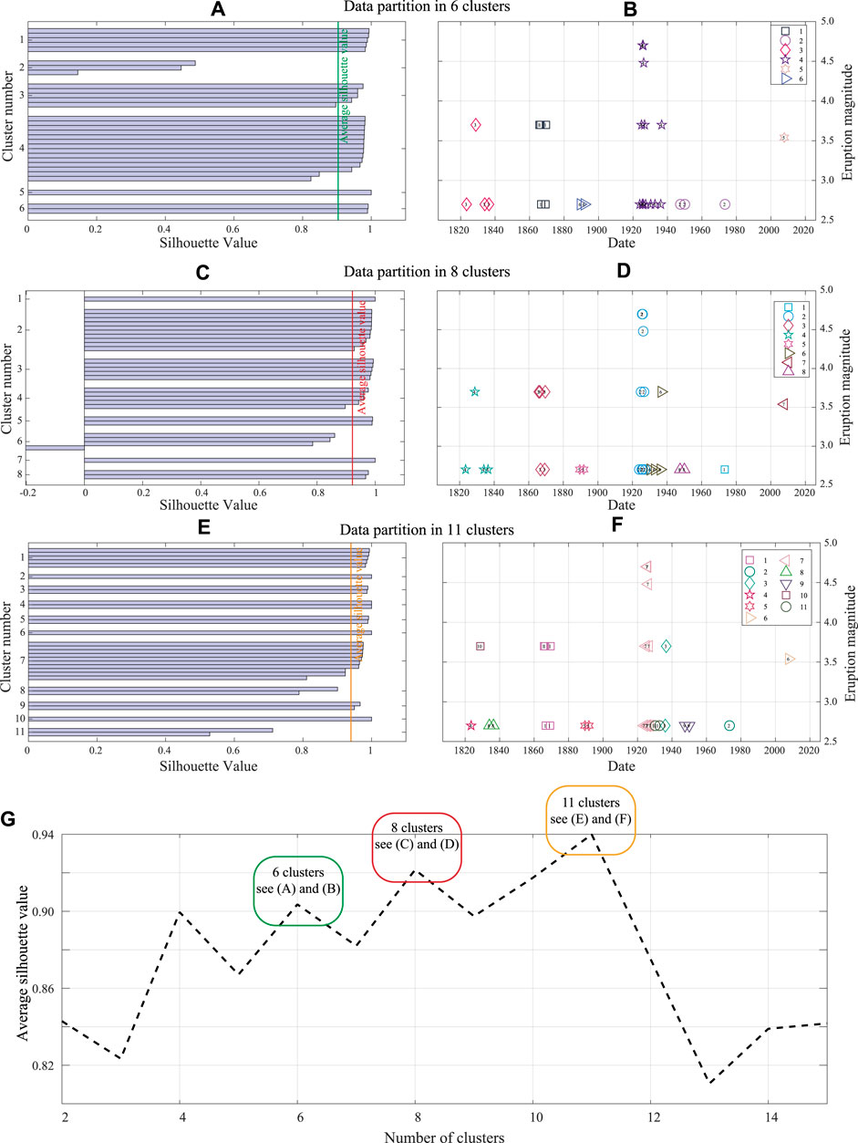
FIGURE 6. Left panel: plot of the silhouette coefficient $s\left(i\right)$ for the partition in 6 (A), 8 (C) and 11 (E) clusters; vertical lines show the average silhouette width. We see that the second cluster in the case of partition in 6 clusters, the sixth in the case of 8, and the 8th and 11th clusters in the case of 11, are below average. In panel C, one of the silhouette values is negative. Right panels: clusters in grouping in time, for partitions in 6 (B), 8 (D) and 11 (F) clusters). Panel (G) shows the average silhouette value for different cluster numbers.

These three possible cluster divisions exhibit high average silhouette values (vertical colored lines in Figures 6A,C,E) indicating relatively good partitions. In the case of 8 clusters however, one of the silhouette coefficients is negative (a negative value means that the event is more similar to the average event in another cluster than in its cluster). In the other two partitions (6 and 11), most of the clusters exhibit silhouette values above the respective average. However, in both cases there are poorly constrained clusters: 1 cluster in the 6-cluster partition and 2 clusters in the 11-cluster partition (Figures 6A–E) show a silhouette value not reaching the average value; furthermore, in the case of 11 clusters, 9 clusters consists of only one or two events having M $\ge$ 2.6.

Taking this latter limitation into account, we choose the simpler 6-cluster partition as the preferred one for analyzing the catalog of Galeras volcano events. Since the choice is ultimately subjective, in Section 6 we will also briefly discuss and compare the results for the alternative eight- and 11-cluster partitions.

Once the clusters are identified, the clusters start times are set using the onset time of the first event within each cluster. The start time of the 6 clusters identified in the Galeras data set (from 1820 and $\text{M}\ge 2.6$) are summarized in Table 2, along with the number of events within each cluster. In the Supplementary Material we provide the same table for the eight- and 11-cluster partitions.

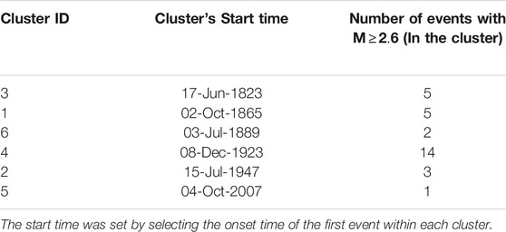
TABLE 2. Selected start time of the 6 clusters identified using the cluster analysis.

Stochastic Modeling of Inter-cluster and Intra-cluster Eruptive Behavior

Figure 7 shows the Cumulative distribution (CDF) of both the inter- and intra-cluster IETs, and the different models tested on the two datasets, in the case of 6-cluster partitioning, and considering the censoring data.

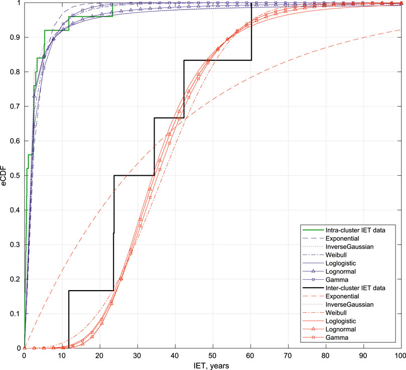
FIGURE 7. Cumulative distribution (CDF) of the data (inter- and intra-cluster) and the different models tested (Exponential, Weibull, Log-logistic, Lognormal, Gamma and BPT) considering the 6-clusters partition.

Table 3 shows a summary of the AIC values obtained for the different alternative models tested for describing the inter-cluster IETs (i.e., long-term process). In bold we highlight the preferred model, with lower AIC, that is the BPT.

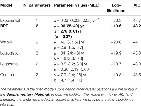
TABLE 3. Competing models tested for describing the inter-cluster time intervals (long term process) considering the 6-clusters partition %.

Table 4 shows a summary of the AIC values obtained for the different competing models tested for describing the intra-cluster IETs (i.e., short-term process). In bold we highlight the preferred model, with lower AIC, that is the Lognormal, as in the “all IETs together” case. This similarity (in terms of model type, and consistency in the best-fitting parameter values) can be explained by the fact that the two datasets used for these two analyses are composed by the same data except the IETs between the pairs of events marking the end of a cluster and the beginning of the successive one. Given the low number of clusters (6), it means there are only five IETs less in the intra-cluster dataset with respect to the “all IETs together” one.

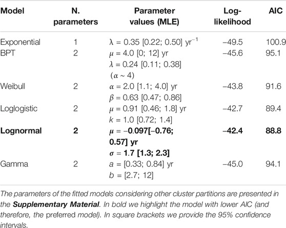
TABLE 4. Competing models tested for describing the intra-cluster time intervals (long term process) considering the 6-clusters partition %.

5.2 Frequency-Size Analysis

For each of the two subsets of possible complete datasets considered in this work (that is, subset 1 (S1): eruptions since 1820 with $M_c\ge 2.6$; subset 2 (S2): eruptions since 1990 with $M_c\ge 1.5$; see Figure 3) we apply the magnitude randomization procedure using the transformation shown in Eq. 4; in practice, we subtract $M_c-\text{Δ}M/2$ to each magnitude value, and sum an ε randomly sampled from an uniform distribution in the interval [-0.05; 0.05] (assuming $\text{Δ}M=0.1$). The Lilliefors test does not reject the null hypothesis of magnitudes being exponentially distributed for the S2 dataset (p-value $\gg 5\%$), where magnitudes are more precisely assessed. For the S1 we need to apply a larger noise to the estimated magnitudes in order to not reject the null hypothesis (with $\text{Δ}M/2=0.2$ or larger, up to 1 unit of magnitude, p-value is always $>5\text{\%}$). This is very reasonable, considering that these are older eruptions and the estimated magnitude is affected by larger uncertainty. By applying the maximum likelihood method we obtain consistent estimates of the b-value for the two datasets (Figure 3): $b_{\text{part }1}=0.86\pm 0.16$ and $b_{\text{part }2}=0.93\pm 0.23$.

5.3 Time-Predictable and Size-Predictable Models

Figure 8 shows the plots of the total erupted mass against the time to the subsequent EEE (Figure 8A) or the time since the preceding EEE (8b) considering the data of each single event independently. In these two cases, the data are not fit by any significant TPM nor SPM model.

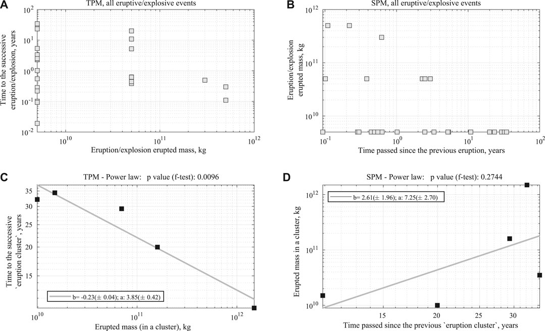
FIGURE 8. (A) Plot of the relationship between time to subsequent eruptive event against the erupted mass (as for a time-predictable model) at a given time and considering each individual event. (B) Plot of the relationship between erupted mass at a given time against the time from the previous eruptive event (as for a size-predictable model) and considering each individual event. (C) The same as (A) but considering cluster events (i.e., time to subsequent cluster and the cumulative mass during a cluster and considering the 6-clusters partition). (D) The same as (B) but considering cluster events (i.e., cumulative mass during a cluster and time from previous cluster and considering the 6-clusters partition).

We perform the same analysis for the clustered EEEs; in this case, the erupted mass in a given cluster is plotted against the time from the end of that cluster to the start of the subsequent one (8c) or the time between the end of the previous cluster and the onset of the one erupting that mass(8 days). According to the plot in Figure 8C, there is some evidence (p-value of F-test: 0.0096) for a possible “inverse” time-predictable relationship in which eruption clusters characterized by large erupted mass are followed by shorter repose times (until the start of the following eruptive cycle). The fitted model shown in Figure 8C implies a power law relationship between time to the subsequent cluster and erupted mass:

where $\beta =-0.23\left(\pm 0.04\right)$ (f-test with ${\text{H}}_0$: $b=0$ is rejected with p-value $\ll 1\text{\%}$), and $\alpha =3.9\left(\pm 0.4\right)$. According to this model, in case the current cluster does not resume to activity of magnitude 2.6 or above, given the present mass output from the 2007 eruption, we should expect about 30 years (from 2007) for the next cluster to start.

6 Discussion

A new catalog of eruption explosive events at Galeras was collated by using the datasets from the Colombian Geological Survey and data from the Smithsonian Institution.

We consider that the catalog is complete, stationary and composed by independent events since 1820, for events with $M\ge 2.6$. This catalog, taking it as a whole dataset of the realization of a homogeneous point process, is best fitted by a Lognormal model, implying that the logarithm of the IETs, taken all together, are normally distributed. The μ parameter of the Lognormal distribution represents the mean of the natural logarithm of the cataloged IETs, so that $e^{\mu }$ is their geometric mean; the latter can be taken as a characteristic timescale, which in this case has a value of approximately 1.6 years. However, being a geometrical mean, its value is strongly influenced by the shortest IETs.

Along with the CV value, some of the fitted distributions to the IETs all together have parameters pointing at a clustering of the EEE. For example, the parameter $\alpha =\sqrt{\mu /\lambda }$ in the BPT model (reported in Table 1) is an indicator of the aperiodicity of the process (Garcia-Aristizabal et al., 2012) and here has a value much larger than 1, as does the ß-value of the Weibull model. These indicators support the visual observation of clustering in the EEE occurrence. Thus, we are able to identify different plausible cluster partitions. From these, the partition into 6 clusters seems to be the one providing the best trade off in the distance measures used for grouping the events and therefore we take this one as the reference partition for the discussion. Nevertheless, in both the main text and the Supplementary Material we complement the description presenting the respective analogue results obtained when using a different partition.

Considering the recurrence analysis of the eruptive events within an eruptive cycle, the preferred stochastic model describing the intra-cluster time intervals for this data set is the Lognormal (integrating the data from all the clusters), with a characteristic timescale parameterized by the μ parameter, translating into a geometrical mean of intra-cluster IETs of approximately 0.9 years. From Table 4 we see that a comparable fit is achieved by the LogLogistic distribution, with the same characteristic time scale (again representing the geometrical mean).

Conversely, considering the recurrence analysis of the eruptive cycles (i.e., long-term process), the preferred stochastic model describing the inter-cluster time intervals is the BPT, with a characteristic repose time (scale parameter) of approximately 36 years. The parameter α shown in Table 3 in the present case takes a value around 0.4, which indicates a slight tendency toward periodical behavior (see e.g., Garcia-Aristizabal et al., 2012). Although the BPT is the preferred model, all the other distributions except the Exponential fit the data similarly. Such similar values of the LogLikelihood are due also to the low number of clusters available in the record. In any case, we keep the BPT as the model best-explaining the inter-cluster onset times.

As mentioned in Section 4, in a history-dependent point process, the conditional probability that an event happens in a time interval $\left(x,x+\text{Δ}t\right)$, given an interval of $x=\left(t-t_L\right)$ years since the occurrence of the previous event (with t the current time of the assessment, and $t_L$ the time of the last event, so that x is the time from the last event), is the hazard rate or hazard function. The hazard function describes instantaneous failure rate, or in other words the conditional probability density of failure at time t given that no event occurred in the time interval x. An increasing hazard function at time t indicates that an event is more likely to occur in a given increment of time $\text{Δ}t$ than it would be in the same increment of time in an earlier age. The hazard function describing the probability to experience the next event in the time interval $\left[x;x+\text{Δ}t\right]$ given no event has occurred in x (that is again the time elapsed since the last event) can be calculated as follows:

where T is the occurrence time of the next event, $f\left(x\right)$ is the probability density function and $F\left(x\right)$ is the cumulative distribution.

The implications of the different results in terms of renewal processes, found so far, can be analyzed inspecting the hazard rate function (see Figure 9A; in the Supplementary Material we provide the same plot for the 8- and 11-cluster partitions). The hazard rate of the Lognormal distribution fitted to all the IETs (without considering clustering of events) is a sharp increasing and then slowly decreasing function. It broadly means that the conditional probability of a new event is high shortly after an event, and slowly decreases as time progresses. This is a clear indication of a clustering effect. Given the current information that no $M\ge 2.6$ event has occurred during the current censoring time x (approximately 12 years, since 4th October 2007), the probability of such an event in the next year can be calculated by Eq. 6 (Garcia-Aristizabal et al., 2012), with $\text{Δ}t$ = 1 year. By using the best fitting model parameters from Table 1, we have a probability of about 6% in the year 2020. In Figure 10 (Box A) we also give an idea on how well this estimate is constrained: by sampling the Lognormal parameters within their uncertainties (from a bivariate Normal distribution and accounting for their covariance), we recalculate the probability of a new EEE in the year 2020. The 95% confidence interval for the probability of a new EEE in 2020 under this model ranges from 4 to 10% (Panel A1).

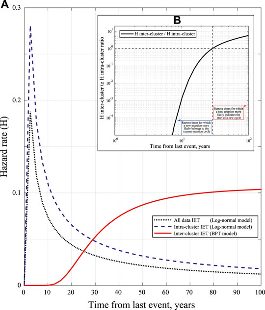
FIGURE 9. Panel A: Hazard function of the BPT distribution selected as the preferred model for describing the inter-cluster time intervals (i.e., time periods between the onset of eruptive cycles), the Lognormal model selected as the preferred model for describing the intra-cluster IETs (in both cases, considering the 6-clusters partition), and the Lognormal model describing all the IETs together without partition into cluster. Inset B: ratio of the inter-to the intra-cluster hazard function given in panel A, highlighting the complementary domains over which the two processes are more likely to explain repose times.

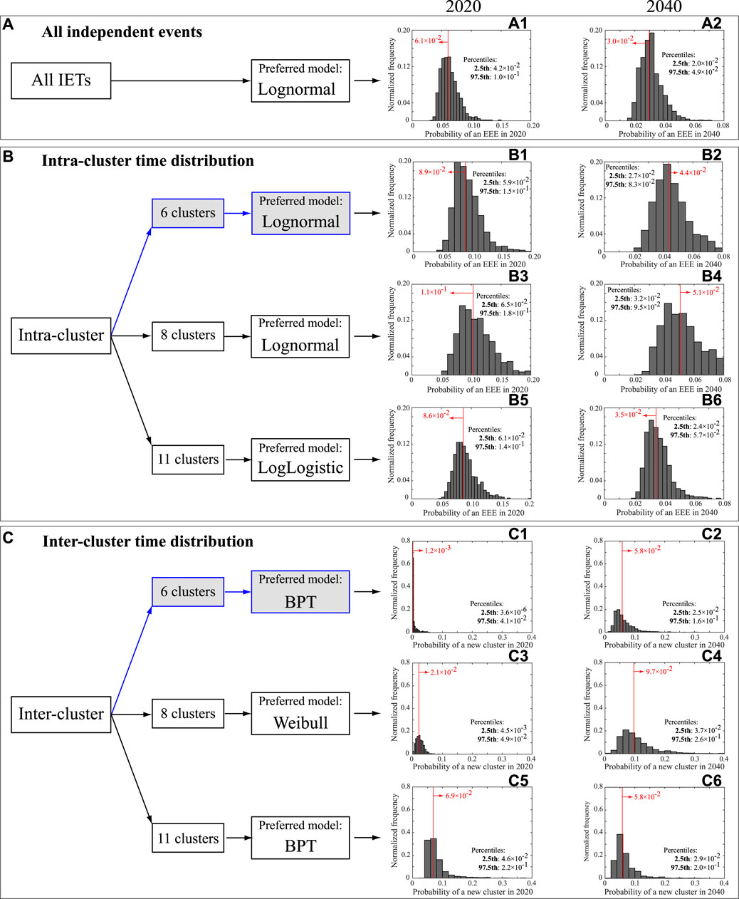
FIGURE 10. Summary of the probability for a new EEE (Boxes A and B) or a new cluster (Box C) in the year 2020 (left-column histograms) or 2040 (right-column histograms) given no new explosive event after the 2007 one. The three Boxes summarize the different data analyzed (all IETs together, intra-cluster IETs and inter-cluster time intervals, respectively in A, B and C). For the intra- and inter-cluster models, we provide the preferred model selected by AIC (see also Tables 3 and 4) when considering different cluster partitions (our preferred partition on 6 clusters is highlighted in gray). The histograms in panels (A1) to (C6) have been obtained by sampling 1,000 times the preferred-model parameters within their uncertainty range (considering covariance when the parameters are more than one) and thus calculating 1,000 values for the probability. In red we give the probability resulting from the best-fit model parameters, and in each panel we also give the 2.5th and 97.fifth percentiles of the 1,000 values to show the 95% confidence interval.

We can use the analysis of cluster to assess how likely a new event would belong to the ongoing cluster, or would mark the onset of a new cluster. The analysis on the 6-cluster partitioned data shows that the hazard rate function best describing the intra-cluster IETs distribution is again a Lognormal distribution, similar to the “all IETs together” one: the longer the time from the last events within a cluster, the lower the likelihood of having a new event. This well describes the gradual decline of activity during an eruptive cycle. Given the current repose time of about 12 years since the last event in the last cluster, the probability of a new M $\ge$ 2.6 in the year 2020 is about 9%, quite similar to the one obtained considering “all IETs together”. This is reasonable, considering the similarity between the two datasets (see Section 5.1.2). In Figure 10 (Box B) we see that the 95% confidence interval for the probability of a new EEE in 2020 belonging to the current cluster spans from 6 to 15% (Panel B1).

The preferred model describing the inter-cluster time intervals is a BPT, which can be seen as a delayed Poisson process: in our case, the hazard rate is very small for about 15 years after an eruptive cycle has begun (Figure 9A), and increases monotonically up to around 65 years, when it becomes flat as in the case of a homogeneous Poisson process, characterized by a constant hazard rate (e.g., Garcia-Aristizabal et al., 2012). The probability of a new eruptive cycle beginning becomes non negligible after a time passed since the start of the previous cycle of about 16 (or 20) years, i.e., when the survivor function is smaller than 99% (or 95%). Given the current elapsed time since the beginning of last cluster of about 12 years, there is a probability of about 0.1% of entering in a new eruptive cycle in the year 2020. In Figure 10 (Box C) we see that the uncertainty on the BPT parameters propagates into a 95% confidence interval on such value that spans from ∼0 to 4% (Panel C1).

A question we may try to answer is when to consider a cycle over, once Galeras is in an eruptive cycle, according to the clustered model for $M\ge 2.6$ events. By using the fitted model parameters for the 6-cluster partition in the intra-cluster Lognormal model (Table 4), a repose of about 47 and 15 years yields respectively a 1 and 5% probability in the survivor function.

These results suggest that, overall, at present we are more likely still in the cluster that started in 2007: in other words, if the volcano re-enters in activity with $M\ge 2.6$ or above during the current year (2020), according to this clustering model this EEE would be more likely associated to the ongoing eruptive cycle, rather than to the start of a new eruptive cycle. Speculatively, a slightly different judgment would be given in case no EEE occurs in the next 20 years approximately, i.e., until the year 2040: in such case, the probability in that year to experience an EEE overall from the “all IETs together” model would be about 3%, and similarly of an EEE belonging to the present cluster (4%), while the probability of an EEE opening a new cluster becomes about 6%. This is just an example to show how the results from the cluster model can be interpreted, keeping separate the intra- and inter-cluster models. In the right-column panels of Figure 10 we show the resulting probability for an event in year 2040, under different models, accounting for the uncertainty on the model parameters. The respective 95% confidence intervals for the three probabilities are (2–5), (3–8) and (3–18)% (Panels A2, B2 and C2, respectively).

Overall, when considering the “all IETs together” (as well as the intra-cluster) modeling, we obtain a best-fitting model that describes a decreasing hazard rate (Figure 9A) in time. This implies that, after a long time has elapsed since the last event of $M\ge 2.6$, the eruptive activity tends to vanish. In this view, the cluster model, through the description of inter-cluster time intervals, is useful to describe the recognized long-term behavior of Galeras, characterized by time-separated eruptive cycles at least in the last 200 years. As shown in Figure 9B, where we plot the ratio of the inter-to the intra-cluster hazard rate, the hazard rates for these two processes are comparable for a censoring time of approximately 30 years, a sort of threshold for discriminating which of the two processes is more likely to be the origin of the current censoring time.

In order to account for the subjectivity in the cluster partitioning, in Figure 10 we show the same results for the 8- and 11-cluster partitioning. In particular:

• The intra-cluster preferred model is again the Lognormal for the 8-cluster partitioning, and the LogLogistic for the 11-cluster one, with comparable distribution parameters and resulting probability for a new intra-cluster EEE in 2020 or 2040 (due to the same reason for the similarity between the “all IET together” and 6-cluster cases, panels B3, B4, B5 and B6).

• The 8-cluster partitioning favors a Weibull model for the inter-cluster time occurrence (Panels C3 and C4), while the 11-cluster partitioning favors again a BPT (panels C5 and C6) as in our preferred 6-cluster one. However we notice that the difference in the probability for a new cluster in 2020 is much more pronounced for the 11-cluster case (best value and 95% confidence interval respectively 7 and (4–20)%, panel C5) than in the 8-cluster case (2 and (0.5–5)%, panel C3), compared to our preferred 6-cluster partitioning. Clearly, a different definition of clusters heavily influences the model describing the inter-cluster distribution, and in particular, the higher the number of identified clusters, the shorter their inter-time. In any case, the three different partitions do not provide dramatically different values for the speculative example of a new cluster in 2040, given no further EEE the last one in 2007: respectively for the 8- and 11-cluster cases, we find such probability to be 10 and 6%, with 95% confidence intervals (4–29)% and (3–19)% (Panels C4 and C6 respectively).

The approach adopted here to purely describe the intra- and inter-cluster occurrences in the catalog has a remarkable limitation: both the distributions adopted for the two processes share the same time domain (that is the entire real axis both for IETs within and among clusters). This limitation does not allow us proposing a single merged model for eruption forecasting based on the clustering approach. In principle, it would be possible to overcome this limitation and create a single consistent model by truncating the IET distributions over separate time domains for the inter- and intra-cluster intervals. However, a major problem of such a model in the present case, characterized by few tens of data, would be to set the time boundaries necessary to truncate the two distributions in a meaningful and robust procedure. This is the reason why we prefer not to truncate them, and stick to a description of the catalog occurrences within the two identified regimes, separately.

The frequency-size analysis, although performed on a dataset restricted to the last few decades of activity, returns b-values that are consistent when considering two separate subsets of the catalog, spanning different periods of time and magnitude range. This indicates a common power law on the erupted mass, linking eruptions of different scale and energy in a scale-invariant relationship, and implying that there is no characteristic size in the eruptive process. We acknowledge that this is not a sufficient proof, but only a possible hypothesis not confuted by the data we have available at this stage.

In principle, we could apply the frequency-size analysis to the clustered data, to find a distribution for the cluster magnitude (i.e., the total erupted mass in an eruptive cycle), as in the time- and size-predictable analysis. However, we objectively identified only 6 clusters, and this number is too low to compute a b-value. However, this would represent an innovative analysis in eruption catalogs, and we recommend it as a possible future work for detailed volcanic records in which many clusters can be isolated.

Finally, we have found that the logarithm of the total erupted mass in an eruption cycle shows a significant inverse linear relationship with the time to the following eruption cycle. In other words, the higher the total erupted mass during an eruptive cycle, the shorter the time until the start of the successive eruption cycle. According to this model, if the current cluster will not experience a mass output much larger than the present output (from the 2007 eruption) we should expect about 18 years from now (or about 30 years from last EEE with magnitude ≥2.6 in 2007) for the next cluster to start. It is interesting to note that this time is similar to the one required by the inter-cluster model for a new cluster to begin (survivor larger than 5%), and larger than the probability of an intra-cluster EEE.

Many of the results found in this study on Galeras may be explained by a simple conceptual model of a volcanic system fed by two interconnected shallow and deep magma reservoirs, as already proposed for e.g., Soufriere Hills, Montserrat (Melnik and Costa, 2014), or Colima, Mexico (Massaro et al., 2019). The deep reservoir feeds the shallow one through a dyke-like structure, and the magma transfer from the deep to the shallow reservoir is strongly controlled by the pressure gradient between the two reservoirs. An eruptive cycle (originating events that determine the intra-cluster IETs) starts when the magma in the shallow reservoir overcomes a threshold in a state variable, for example the overpressure, which can be the result of renewed magma fed from the deeper reservoir. Meanwhile, the long-term recharging of the system (originating the inter-cluster time intervals), which can be primarily modulated by the pressure gradient between the two reservoirs, may take place in the background; magma flux from the deeper chamber is likely stimulated as the pressure gradient increases while an eruptive cycle goes on, revitalizing the system to start a new eruptive cycle. When looking at the all IETs together, we best explain the IETs by a Lognormal distribution characterized by a mean linked to the geometrical mean of the IETs, and by a thick tail that accounts for longer reposes, characteristic of the times between the last event in a cycle and the first event of the subsequent one. The erupted mass in each event does not show a preferred size. However, when considering clustering, we best explain the inter-cluster onset times by a BPT model. Such model is usually interpreted as a realization of a point process in which new activity will occur when a threshold is reached, the overpressure of the shallow reservoir in our case. In the time between two eruptive cycles, the shallow system is recharged by the deep one: this reloading is governed by two components, that are a constant-rate loading component (also called the drift term, for example a constant-rate recharging from the deep to the shallow reservoirs) and a random component (also termed Brownian motion) that may be due to random stress perturbations on the reservoir system (for example in terms of variations in the stress field due to regional seismicity or activity at other nearby volcanoes, or variations in the deep recharging process). The latter component may thus randomly disturb the volcanic system causing an aperiodicity in the mean repose time between eruptive cycles, although in the case of Galeras we have found that this aperiodicity is weak. The inverse TPM found for Galeras tells us that the eruptive cycles characterized by a large total erupted mass can create a higher pressure gradient between the deep and the shallow reservoirs, favoring the flux of magma feeding the shallow reservoir. Conversely, eruptive cycles with a low total erupted mass do not significantly perturb the pressure in the shallow chamber, hence the pressure gradient between the two reservoirs, inhibiting the “eruptability” of shallow magma.

7 Conclusion

We have analyzed a catalog of explosion events at Galeras volcano, with different perspectives, to extract the significant features of event occurrence when considering onset times, eruption magnitudes, and the two together.

We first identify as complete the part of the catalog from 1820 with eruption magnitudes 2.6 or larger.

On this complete catalog, the IETs are best described by a Lognormal model, with a characteristic IET of about 1.6 years. However, there is a clear tendency for explosion events to cluster in time, originating eruptive cycles. The identification of such cycles is inherently subjective: by adopting a set of reasonable criteria, we identify a preferred partitioning of the events from 1820 with magnitude $\ge$ 2.6 into 6 clusters. Under this partitioning, the distribution of events within a cycle is best explained by a Lognormal distribution, while onset times between clusters are best explained by a Brownian Passage Time model, that can be seen as a delayed Poisson process. The added value of the clustered model lies in its ability to describe the re-activation of volcanic activity, through the modeling of inter-cluster time intervals, with respect to the best-fitting model on all the IETs together: this latter model forecasts a gradual decline in the probability of a new event, after an initial peak, which would unrealistically lead to a vanishing of the explosive activity in case no event occurs for a prolonged period.

The eruption magnitudes of single eruptive events seem to be governed by a power law distribution, implying that there is no characteristic size for single events.

However, when considering the time between eruptive cycles and the volume erupted during each cycle, we observe an inverse time-predictability: the larger the volume erupted in the previous cycle, the shorter we will have to wait for a new cycle to begin.

These results suggest a simple conceptual model, consisting of a plumbing system characterized by two magma reservoirs located at different depths and connected by a dike system. In this model, the deep storage feeds magma into the shallow one through a constant-rate process that is randomly perturbed (for example by regional or local stress variations), triggering a new cycle onset when a threshold in the overpressure of the shallow reservoir is reached: a cluster of events in time occurs, consisting of many small events or few large ones (following, in general, a power-law distribution), relaxing in turn the shallow reservoir. If the total erupted volume in the cycle is large, it favors the uprizing of new magma from the deep reservoir to the shallow one by an increased pressure gradient between the two. In this way, the waiting time for a new cycle to begin is shorter.

According to the monitoring observations of the Servicio Geologico Colombiano (SGC), along with no significant eruptive activity at Galeras in about a decade, there has been also lack of geophysical signals that unambiguously indicate new magma feeding the system. Under this perspective, the last cluster seems to be over, and a new eruptive event could be classified as the first one of a new cluster. However, considering our probability estimates of having either a new eruption in the current cluster or the start of a new cluster next year, the preferred 6-clusters partition indicates a larger probability for a potential new event in the next year as belonging to the previous cluster rather than opening a new one, whereas when considering a 11-cluster partitioning, these two probabilities are very similar. It is worth noting that our analysis strictly focuses on the pure temporal occurrence of events (above a relatively high completeness magnitude), regardless of all the other observables that may further constrain the onset, or the end, of a cluster, such as the presence or absence of seismic activity, deformations, or geochemical anomalies. Including such observations to complement any clustering approach would be of invaluable support for analyzing recent and frequent activity, whereas it is less supportive for a long-term analyses, as the one presented in this article.

Data Availability Statement

The original contributions presented in the study are included in the article/Supplementary Material, further inquiries can be directed to the corresponding author.

Author Contributions

AC, LS and AGa conceived the study and methods used to analyze the Galeras volcano, and have interpreted the results achieved. LS performed the analysis on independent events, and on the frequency-size relationship. AGa carried out the cluster and the size- and time-predictability analyses. LS and AGa wrote the bulk of the text, with input from all co-authors. AGL and GC collated the Galeras dataset and wrote the sections on Galeras volcano and data, and contributed to the discussion of the analysis of the results. All the authors have read and approved the manuscript.

Funding

This research has been partially funded by project EXACT (Progetto 29 di Ricerca Libera INGV 2019 Delibera 53/2020).

Conflict of Interest

The authors declare that the research was conducted in the absence of any commercial or financial relationships that could be construed as a potential conflict of interest.

The handling editor declared a past co-authorship with several of the authors (LS, AC).

Acknowledgments

AC warmly thanks the Servicio Geologico Colombiano and the Universidad de Narino for inviting him to visit the Observatorio Vulcanológico y Sismológico de Pasto and hosting him during his stay in Colombia.

Supplementary Material

The Supplementary Material for this article can be found online at: https://www.frontiersin.org/articles/10.3389/feart.2020.583703/full#supplementary-material.

References

Aki, K. (1965). Maximum likelihood estimate of b in the formula log (n) = a bm and its confidence limits. Bull. Earthquake Res. Inst. Univ. Tokyo 43, 237–239.
Al-Zoub, M., and Al Rawi, M. (2008). An efficient approach for computing silhouette coefficients. J. Comput. Sci. 43, 252–255. doi:10.3844/jcssp.2008.252.255
Bain, L. J. (1978). Statistical analysis of reliability and life-testing models, theory and methods. New York: Marcel Dekker.
Bebbington, M. S., and Cronin, S. (2011). Spatio-temporal hazard estimation in the auckland volcanic field, New Zealand, with a new event-order model. Bull. Volcanol. 73, 55–72. doi:10.1007/s00445-010-0403-6
Bebbington, M. S. (2008). Incorporating the eruptive history in a stochastic model for volcanic eruptions. J. Volcanol. Geoth. Res. 175, 325–333. doi:10.1016/j.jvolgeores.2008.03.013
Bebbington, M. S., and Lai, C. D. (1996). On nonhomogeneous models for volcanic eruptions. Math. Geol. 28, 585–600.
Bebbington, M. S. (2012). Models for temporal volcanic hazard. Statistics in Volcanology 1, 1–24. 10.5038/2163-338X.1.1.
Bebbington, M. S. (2010). Trends and clustering in the onsets of volcanic eruptions. J. Geophys. Res. 115, B01203. doi:10.1029/2009JB006581
Bevilacqua, A., Flandoli, F., Neri, A., Isaia, R., and Vitale, S. (2016). Temporal models for the episodic volcanism of campi flegrei caldera (Italy) with uncertainty quantification. J. Geophys. Res. Solid Earth 121, 7821–7845. doi:10.1002/2016JB013171
Bolshakova, N., and Azuaje, F. (2003). Cluster validation techniques for genome expression data. Signal Process. 83, 825–833. doi:10.1016/S0165-1684(02)00475-9
Bonadonna, C., and Costa, A. (2013). Plume height, volume, and classification of explosive volcanic eruptions based on the weibull function. Bull. Volcanol. 75, 742. doi:10.1007/s00445-013-0742-1
Burt, M. L., Wadge, G., and Scott, W. A. (1994). Simple stochastic modelling of the eruption history of a basaltic volcano: nyamuragira, Zaire. Bull. Volcanol. 56, 87–97. 10.1007/BF00304104.
Calvache, M. L., Cortés, G. P., and Williams, S. N. (1997). Stratigraphy and chronology of the Galeras volcanic complex, Colombia. J. Volcanol. Geotherm. Res. 77, 5–19. doi:10.1016/S0377-0273(96)00083-2
Calvache, V. M. L. (1990). Geology and volcanology of the recent evolution of Galeras Volcano, Colombia. Master’s thesis. Baton Rouge: Louisiana State University.
Cepeda, H. (2020). Quinientos años de documentacioÌn histoÌrica de actividad del volcaÌn Galeras: escenarios eruptivos (Servicio GeoloÌgico Colombiaon).
Chen, G., Jaradat, S. A., Banerjee, N., Tanaka, T. S., Ko, M. S. H., and Zhang, M. Q. (2002). Evaluation and comparison of clustering algorithms in analyzing es cell gene expression data. Stat. Sin. 241–262.
Coles, S., and Sparks, R. (2006). “Extreme value methods for modeling historical series of large volcanic magnitudes,” in Statistics in Volcanology. Editors H. Mader, S. Coles, C. Connor, and L. Connor (London: Geological Society IAVCEI Publications), 47–56.
Connor, C. B., Sparks, R. S. J., Mason, R. M., and Bonadonna, C. (2003). Exploring links between physical and probabilistic models of volcanic eruptions: the soufriere hills volcano, Montserrat. Geophys. Res. Lett. 30, 1701. doi:10.1029/2003GL017384
Conway, F. M., Connor, C. B., Hill, B. E., Condit, C. D., Mullaney, K., and Hall, C. M. (1998). Recurrence rates of basaltic volcanism in sp cluster, san francisco volcanic field, Arizona. Geology 26, 655–658. doi:10.1130/0091-7613(1998)026 (0655:RROBVI) 2.3.CO;2
Cronin, S., Bebbington, M., and Lai, C. (2001). A probabilistic assessment of eruption recurrence on taveuni volcano, Fiji. Bull. Volcanol. 63, 274–288. doi:10.1007/s004450100144
DANE (2011). Estimación y proyección de población nacional, departamental y municipal total por área 1985-2020. Tech. Rep. Bogotá: Departamento Administrativo Nacional de Estadística.
De la Cruz-Reyna, S. (1991). Poisson-distributed patterns of explosive eruptive activity. Bull. Volcanol. 54, 57–67.
Deligne, N., Coles, S., and Sparks, R. (2010). Recurrence rates of large explosive volcanic eruptions. J. Geophys. Res. 115, B06203. doi:10.1029/2009JB006554
Espinoza, B. A. (1988). Actividad de1 volcán Galeras en épocas históricas. Tech. Rep. 80 [in Spanish].
Furlan, C. (2010). Extreme value methods for modelling historical series of large volcanic magnitudes. Stat. Model. Int. J. 10, 113–132. doi:10.1177/1471082X0801000201
Garcia-Aristizabal, A., Bucchignani, E., and Manzi, M. P. (2017). Patterns in climate-related parameters as proxy for rainfall deficiency and aridity: application to Burkina Faso. ASCE-ASME J. Risk Uncertain. Eng. Syst. A. 3, A4016001. doi:10.1061/AJRUA6.0000860
Garcia-Aristizabal, A., Marzocchi, W., and Fujita, E. (2012). A Brownian model for recurrent volcanic eruptions: an application to Miyakejima volcano (Japan). Bull. Volcanol. 74, 545–558. doi:10.1007/s00445-011-0542-4
Garcia-Aristizabal, A., Selva, J., and Fujita, E. (2013). Integration of stochastic models for long-term eruption forecasting into a Bayesian event tree scheme: a basis method to estimate the probability of volcanic unrest. Bull. Volcanol. 75, 1–13. doi:10.1007/s00445-013-0689-2
Global Volcanism Program [Dataset] (2013). Version. 4.9.1. “Galeras (351080),” in Volcanoes of the World. Editor E. Venzke (Washington, DC: Smithsonian Institution).
Gutenberg, R., and Richter, C. (1944). Frequency of earthquakes in California. Bull. Seismol. Soc. Am. 34, 185–188.
Hurtado Artunduaga, A. D., and Cortés Jiménez, G. P. (1997). Third version of the hazard map of Galeras Volcano, Colombia. J. Volcanol. Geoth. Res. 77, 89–100. doi:10.1016/s0377-0273(96)00088-1
INGEOMINAS (2010). Technical Reports. Resumen de actividad del volcan galeras del 29 de diciembre de 2009 al 4 de enero de 2010. Observatorio vulcanológico Y sismológico de pasto resumen. INGEOMINAS.
INGEOMINAS (2005). Technical Reports. Volcán Galeras Actividad histórica. INSTITUTO COLOMBIANO DE GEOLOGIA Y MINERIA INGEOMINAS.
Kaufman, L., and Rousseeuw, P. J. (2008). Finding Groups in Data: An Introduction to Cluster Analysis. John Wiley & Sons.
Klein, F. (1982). Patterns of historical eruptions at Hawaiian volcanoes. J. Volcanol. Geoth. Res. 12, 1–35. doi:10.1016/0377-0273(82)90002-6
Lilliefors, H. (1969). On the Kolmogorov-smirnov test for the exponential distribution with mean unknown. J. Am. Stat. Assoc. 64, 387–389.
MacQueen, J. (1967). “Some methods for classification and analysis of multivariate observations,” in Proceedings of the fifth berkeley symposium on mathematical statistics and probability. Berkeley, California: University of California Press, Vol. 1, 281–297.
Marzocchi, W., and Sandri, L. (2003). A review and new insights on the estimation of the b -value and its uncertainty. Ann. Geophys. 46, 1271–1282. doi:10.1002/2016JB013054
Marzocchi, W., Sandri, L., Heuret, A., and Funiciello, F. (2016). Where giant earthquakes may come. J. Geophys. Res. Solid Earth 121, 7322–7336. doi:10.1002/2016JB013054
Marzocchi, W., and Zaccarelli, L. (2006). A quantitative model for time-size distribution of eruptions. J. Geophys. Res. 111, B04204. doi:10.1029/2005JB003709
Mason, B., Pyle, D., and Oppenheimer, C. (2004). The size and frequency of the largest explosive eruptions on earth. Bull. Volcanol. 66, 735–748. doi:10.1007/s00445-004-0355-9
Massaro, S., Costa, A., Sulpizio, R., Coppola, D., and Capra, L. (2019). Cyclic activity of the fuego de colima volcano (Mexico): insights from satellite thermal data and nonlinear models. Solid Earth 10, 1429–1450. doi:10.5194/se-10-1429-2019
Melnik, O., and Costa, A. (2014). “Dual chamber-conduit models of non-linear dynamics behaviour at soufrière hills volcano,” in The eruption of Soufriere Hills volcano, Montserrat from 2000 to 2010. Editors G. Wadge, R. Robertson, and B. Voight (London: Geological Society of London), Chap. 3, Vol. 39 of 5, 61–69.
Mendoza-Rosas, A., and la Cruz-Reyna, S. D. (2008). A statistical method linking geological and historical eruption time series for volcanic hazard estimations: applications to active polygenetic volcanoes. J. Volcanol. Geoth. Res. 176, 277–290. 10.1016/j.jvolgeores.2008.04.005.
Mulargia, F., Tinti, S., and Boschi, E. (1985). A statistical analysis of flank eruptions on Etna volcano. J. Volcanol. Geoth. Res. 23, 263–272.
Newhall, C., and Self, S. (1982). The Volcanic Explosivity Index (VEI): an estimate of explosive magnitude for historical volcanism. J. Geophys. Res. 87, 1231–1238.
Papale, P. (2018). Global time-size distribution of volcanic eruptions on earth. Sci. Rep. 8, 6838. doi:10.1038/s41598-018-25286-y
Passarelli, L., Sansò, B., Sandri, L., and Marzocchi, W. (2010). Testing forecasts of a new bayesian time-predictable model of eruption occurrence. J. Volcanol. Geotherm. Res. 198, 57–75. doi:10.1016/j.jvolgeores.2010.08.011
Pyle, D. (1998). Forecasting sizes and repose times of future extreme volcanic events. Geology 26, 367–370. doi:10.1130/0091-7613(1998)026(0367:FSARTO) 2.3.CO;2
Pyle, D. (2000). “Sizes of volcanic eruptions,” in Encyclopedia of volcanoes. Editors H. Sigurdsson, B. Houghton, S. McNutt, H. Rymer, and J. Stix (London: Academic Press).
Rousseeuw, P. J. (1987). Silhouettes: a graphical aid to the interpretation and validation of cluster analysis. J. Comput. Appl. Math. 20, 53–65. doi:10.1016/0377-0427(87)90125-7
Sandri, L., Acocella, V., and Newhall, C. (2017). Searching for patterns in caldera unrest. Geochem. Geophys. Geosyst. 18, 2748–2768. doi:10.1002/2017GC006870
Sandri, L., Marzocchi, W., and Gasperini, P. (2005). Some insights on the occurrence of recent volcanic eruptions of Mount Etna volcano (Sicily, Italy). Geophys. J. Int. 163, 1203–1218. 10.1111/j.1365-246X.2005.02757.x.
SGC (2015). Actualización del mapa de amenaza volcánica del volcán galeras—Colombia. Pasto: Servicio geológico Colombiano, Dirección de Geoamenazas.
Simkin, T., and Siebert, L. (2002). GVP-3. Volcanoes of the world: an illustrated catalog of holocene volcanoes and their eruptions. Smithsonian Institution, Global Volcanism Program Digital Information SeriesAvailable at: http://www.volcano.si.edu/world/ (Accessed 2020).
Sobradelo, R., Marti, J., Mendoza-Rosas, A., and Gomez, G. (2011). Volcanic hazard assessment for the canary islands (Spain) using extreme value theory. Nat. Haz. Earth Syst. Sci. 11, 2741–2753. doi:10.5194/nhess-11-2741-2011
Stix, J., Calvache, V. M. L., and Williams, S. N. (1997). Galeras volcano, Colombia interdisciplinary study of a decade volcano. J. Volcanol. Geotherm. Res. 77, 1–4. doi:10.1016/s0377-0273(96)00082-0
Turner, M., Cronin, S., Bebbington, M., and Platz, T. (2008). Developing probabilistic eruption forecasts for dormant volcanoes: a case study from mt taranaki, New Zealand. Bull. Volcanol. 70, 507–515. doi:10.1007/s00445-007-0151-4
UNGRD (2019). Fortalecimiento de la gestión del riesgo de desastres en la zona de amenaza volcánica alta-zava del volcán galeras. (Bogotá, Colombia: Presidencia de la República).
Voight, B. (1989). A relation to describe rate-dependent material failure. Science. 243, 200–203. doi:10.1126/science.243.4888.200
Wickman, F. E. (1966). “Markov models of repose-period patterns of volcanoes,” in Random process in geology. New York: Springer, 135–161.
Keywords: cluster analysis, stochastic modeling, Galeras, inter-event times, time-predictability, size-predictability, frequency-size relationship, eruptive activity
Citation: Sandri L, Garcia A, Costa A, Guerrero Lopez A and Cordoba G (2021) Stochastic Modeling of Explosive Eruptive Events at Galeras Volcano, Colombia. Front. Earth Sci. 8:583703. doi: 10.3389/feart.2020.583703
Received: 15 July 2020; Accepted: 18 November 2020;
Published: 18 January 2021.
Edited by:
Roberto Sulpizio, University of Bari Aldo Moro, ItalyReviewed by:
Mark Bebbington, Massey University, New ZealandEisuke Fujita, National Research Institute for Earth Science and Disaster Resilience (NIED), Japan
Copyright © 2021 Sandri, Garcia, Costa, Guerrero Lopez and Cordoba. This is an open-access article distributed under the terms of the Creative Commons Attribution License (CC BY). The use, distribution or reproduction in other forums is permitted, provided the original author(s) and the copyright owner(s) are credited and that the original publication in this journal is cited, in accordance with accepted academic practice. No use, distribution or reproduction is permitted which does not comply with these terms.
*Correspondence: Laura Sandri, laura.sandri@ingv.it